You're all calculating churn rates wrong
- The false assumption
- What your churn is actually like, with help from K. S. Lomax
- What your churn is actually like, with help from Waloddi Weibull
- Optimizing for a falsehood will lead you astray
- How the h*** do we measure churn then?
- Weibull or Lomax?
- Let's do some proper statistics
- Tail effects: The rare long-term customers make you rich slowly
- Fat tails are nice, but you're blind to them
Many smart people will tell you to obsess over your churn rate.
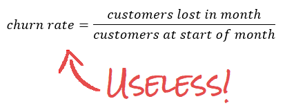
According to Andreessen Horowitz, this number is one of the top 16 metrics to measure a SaaS startup by. Well, sorry Andreessen, and sorry Horowitz, but this just isn't right.
It's counterintuitive, but it's a statistical fact: This number actually tells you nothing useful about churn, but really relates to the age of the subscriptions you have. It will in most cases go down on it's own, and, absurdly, the only way to keep it from going down is to have very high growth. So the number will literally only look bad if your business is doing extremely well, and optimizing for it will be directly counter-productive. The error here is a simple statistical mistake that is easy to make, and luckily also easy to understand and avoid.
If you run a subscription based SaaS business, you're likely very concerned with how long you can keep your customers. We're a JavaScript exception tracking service, and the health of this business is fully determined by how many customers we bring in, and how long we can keep them. On the surface, churn rate may seem like a natural proxy for changes in customer lifetimes. Let's dig into why that is not true.
The false assumption
Computing a churn rate assumes that a customer is equally likely to leave at any time, no matter how long they've been subscribed to you. This is almost certainly not true. In fact, as we will see, having a constant churn probability over time essentially implies that you'll never have long term customers.
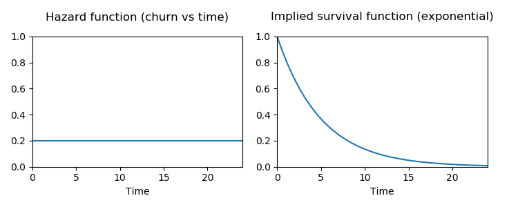
If you have a constant churn of c per month, the probability that a customer stays subscribed for n months is (1-c)^n. This implies that customer lifetimes come from the Geometric distribution. If customers can quit the subscription at any time, we have continuous time and should use the continuous time analogue, the Exponential distribution.
What your churn is actually like, with help from K. S. Lomax
The problem is, your customer is not equally likely to cancel their subscription at any time. Most likely, you have a situation where the drop-off in customers is higher in the first few days than it is later. This is even more so if you have a free trial period for your product.
If the churn probability gets lower the longer the customer has been subscribed, you could model that as c/(t+1), where
t is the timestep (e.g. number of days the customer has been subscribed), and c is some constant.
In this case, this implies that customer lifetimes comes from a Lomax distribution.
This is equivalent to a Pareto distribution shifted to start at 0.

What your churn is actually like, with help from Waloddi Weibull
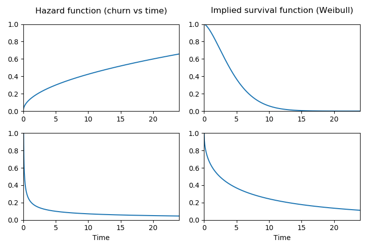
If you suspect that churn probability per day may increase the longer a user has been subscribed, the Lomax distribution won't work for you. Instead you could enlist the help of Swedish statistician Waloddi Weibull. The Weibull distribution can express both decreasing, flat, and increasing probabilities of a customer quitting. This makes it a popular choice for modeling customer lifetimes.
Optimizing for a falsehood will lead you astray
Now let's see why properly modeling this is important.
Let's measure churn the wrong way, and see where it takes us. Let's say customer lifetimes come from a Lomax distribution. Let's also say you have a business that is in terrible shape, where the number of new sign ups per day is falling by one per day. How will this look on the churn rate? We can simulate it and find out.
Keep in mind, in each of the examples below we simulate lifetimes from the same customer lifetime distribution, and this distribution does not change over time.
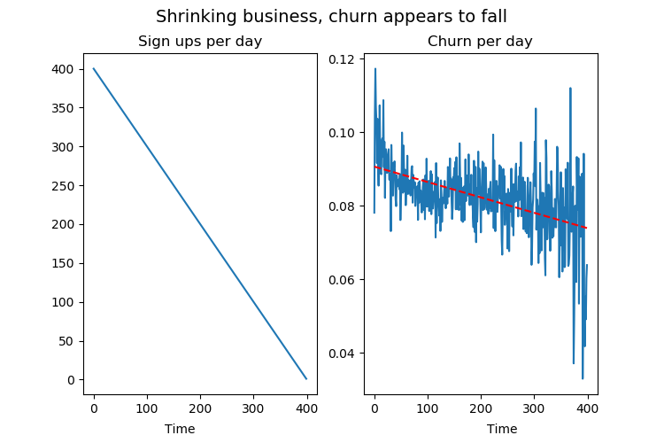
This is clearly a dying business, yet the churn rate graph is looking great! The churn rate per day is falling steadily, even if we know that there is no change in customer lifetimes in our model.
So what's going on? This sharp fall in churn rate is a consequence of the fact that we're not getting new customers. Because we're not growing, a bigger share of our customers have been around for a long time, which means they're less likely to churn, which means our daily churn graph goes down more than it would otherwise. This change on the population level happens despite there being no change in underlying individual customer lifetimes.
Let's change this into a scenario where your business is experiencing insane growth. We'll keep the customer lifetimes exactly the same, but change it so that the number of new sign ups per day is growing superlinearly.
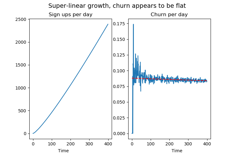
Even if the customer lifetimes are unchanged from before, the churn rate graph here is flat. An investor would frown and say we're doing nothing to improve how well we retain our customers. In reality, the only reason the graph looks "bad" has nothing to do with churn, it is because we're doing insanely well at getting new sign ups.
If you are steering yourself and your team on the basis of this metric, you're rewarding yourself for stifling growth and punishing yourself for growing. Obviously, this is 100% counterproductive.
How the h*** do we measure churn then?
As you might have guessed from the previous paragraphs, we should model the distribution of customer lifetimes, and we should do it in a statistically sound way. Lomax and Weibull distributions are good choices of model.
The part where this gets tricky is that we'll have two types of data: The customers that have quit, and the customers that are still subscribed. It's only our ex-customers that give us a total lifetime to work with. For our still-subscribed customers, we only know that their subscription has lasted up until now, and we don't know how much longer it will last into the future. In statistical lingo, we have what is called right-censored data.
Luckily there's a way to use all our data, even from our still-subscribed customers.
Weibull or Lomax?
Choosing between Weibull or Lomax (or any other distribution) has no simple answer. Weibull is more flexible in that it can express growing, shrinking and flat churn probabilities. However, this expressive power will not help you if your data is fundamentally Lomax-like. First and foremost, base your choice on your knowledge of the business that you're in. If you have any prior knowledge about how churn probabilities will develop, base your choice of distribution on that. There are also various goodness of fit tests you could use to inform this decision. The truth is, any choice of distribution will be wrong to some degree, so you need to make a judgment call as to what fits your situation the best, based both on both your data and your prior knowledge. For the purposes of the rest of this post, we'll just fit both distributions and disregard the question of which suits us the best.
Let's do some proper statistics
The probability distributions we'll model are defined by their parameters. We want to find the parameters that fit the data best. To start, we want to make a guess at these parameters, and have a way to tell how good our guess was. Luckily, we have a statistically sound way of knowing how good a guess is given the data we have. Extra luckily, this is also true when we have censored data. This function that tells us how likely our parameters are given the data we have is called the Likelihood function. We get it by looking up the probability density function value for the uncensored data points and the survival function value for each of the censored data points, and multiplying all these values together.
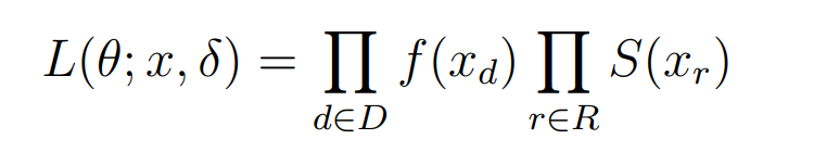
f(.) is the probability distribution function, S(.) is the survival function,
D is the set of uncensored lifetimes and R is the set of right-censored lifetimes.
Next, we remember that computers suck at multiplying numbers close to zero, so we instead take the log of each number and sum them together. We can do this without changing where the function has its maximum. We'll use NumPy and the statistics and optimization packages in SciPy to compute this. Here's the Python code.
import numpy as np
import scipy as sp
import scipy.stats as stats

#duration of alive subscriptions
censored = np.array([133.65, 10.26, 0.24, 3.87, 23.84, 25.91, 41.83, 137.805, 0.985, 100.39, 14.9, 18.72, 29.65, 13.11, 26.71, 22.64, 179.985, 9.6, 37.61, 144.53, 18.855, 80.865, 88.56, 21.955, 73.945, 10.365])
#duration of completed subscriptions
uncensored = np.array([55.31, 47.03, 0.44, 190.41, 80.07, 0.77, 23.93, 151.72, 33.09, 10.9, 140.41, 209.49, 21.38, 40.18, 99.26, 167.52, 16.75, 109.77, 18.07, 90.23, 233.68, 27.09, 42.35, 109.06, 181.86, 24.5, 66.08, 19.25])

#Log likelihoods for censored data
def log_likelihood_weibull(args):
    shape, scale = args
    val = stats.weibull_min.logpdf(uncensored, shape, loc=0, scale=scale).sum() + stats.weibull_min.logsf(censored, shape, loc=0, scale=scale).sum()
    return -val #sign is flipped so we can use a minimizer

def log_likelihood_lomax(args):
    shape, scale = args
    val = stats.lomax.logpdf(uncensored, shape, loc=0, scale=scale).sum() + stats.lomax.logsf(censored, shape, loc=0, scale=scale).sum()
    return -val
Next, we will use a function maximizer to find the parameters that maximize our function L.
(Actually we only have function minimizers, so we'll equivalently minimize -L.)
res_weibl = sp.optimize.minimize(log_likelihood_weibull, [1, 1], bounds=((0.001, 1000000), (0.001, 1000000)))
res_lomax = sp.optimize.minimize(log_likelihood_lomax,   [1, 1], bounds=((0.001, 1000000), (0.001, 1000000)))
What we've just done is called Maximum Likelihood Estimation (MLE). For a more thorough derivation of this estimator under censored data, see this PDF from Daowen Zhang at NCSU.
Now that we have an estimate of the distribution parameters, we can look at the mean and medians of the distribution.
print("weibull shape", res_weibl.x[0], ", scale=", res_weibl.x[1])
print("weibull mean", stats.weibull_min.mean(res_weibl.x[0], scale=res_weibl.x[1]))
print("weibull median", stats.weibull_min.median(res_weibl.x[0], scale=res_weibl.x[1]))

print("lomax shape", res_lomax.x[0], ", scale=", res_lomax.x[1])
print("lomax mean", stats.lomax.mean(res_lomax.x[0], scale=res_lomax.x[1]))
print("lomax median", stats.lomax.median(res_lomax.x[0], scale=res_lomax.x[1]))
This outputs:
weibull shape=1.0935179324818296, scale=122.3601743694174
weibull mean 118.29884582009447
weibull median 87.51413316428012
lomax shape=101.65488165157542, scale=12575.372370928875
lomax mean 124.93554375692996
lomax median 86.03983407302042
The mean tells us the mean customer lifetime, in days. Multiply this by customer income per day, and you have your Customer Lifetime Value.
The median tells us the typical customer lifetime. This is smaller than the mean, because the mean is dominated by the less likely, very large values. The existence of these rarer, very long term customers matter a lot to the outlook of your business, as we will see.
Tail effects: The rare long-term customers make you rich slowly
Let's look at customer survival for two business. Each will have customer lifetimes coming from a Lomax distribution. The distributions will both have the same median customer lifetime, but one has a larger mean lifetime than the other. In other words, one has more long term customers than the other.
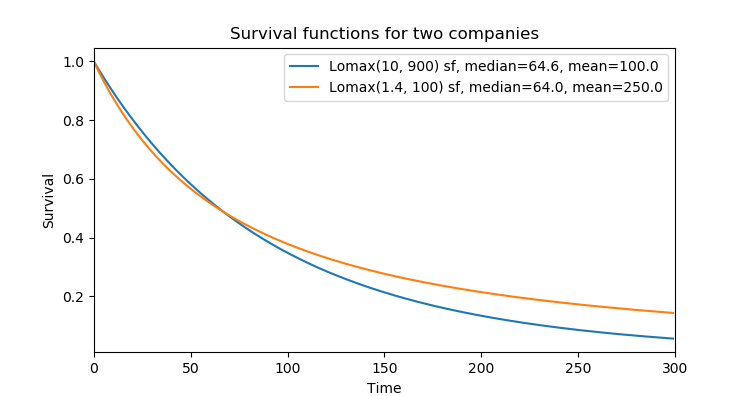
The company following the orange line has higher drop-off of customers in the beginning, but lower drop-off towards the end. The effect on revenue is massive. If you're following the orange line rather than the blue, you're making 2.5 times more money. Keep in mind that the typical customers (found by the median) stick around equally long in either company, but it's the rare long term customers that shift the Lifetime Customer Value massively in favor of the orange company.
Let's simulate the Monthly Recurring Revenue (MRR) for these two businesses. We'll give them each 10 new sign-ups pers month. The difference in the end is massive.
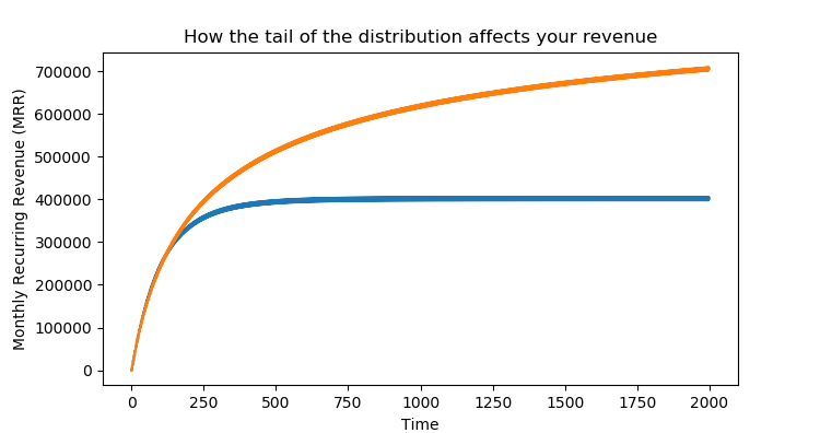
The two companies have similar trajectories in the start, but eventually the effect of the rarer, long term customers show themselves. The orange company will eventually make 2.5x higher MRR than the blue company.
Fat tails are nice, but you're blind to them
Fat tails give you rare events of extreme proportions. In our case it would be rare customer lifetimes that last very long. As we've seen, fat tails in customer lifetime distributions can have massive effects on your long term revenue. However, accurately estimating these turns out to be hard or impossible.
Most people's intuitions fail when it comes to these distributions. Here's an example, due to N. N. Taleb. Let's assume we're dealing with an 80/20 Pareto distribution (or the analogue Lomax(1.13) distribution). Let's say we're computing the sample mean. Where it takes 30 observations for a Gaussian to stabilize the mean up to a given level, it takes 1011 observations from the Pareto to bring the sample error down by the same amount. So if you have Pareto 80/20 distributed customer lifetimes, you need 100 billion customers before the sample mean lifetime is accurate. Good luck! (Note that this is for the sample mean, i.e. summing sample lifetimes and dividing by count. It does not directly apply to the ML estimator we've made above.)
While your customer lifetimes might not follow such an extreme distribution, it serves to make the point that if the tail is sufficiently fat, getting proper estimates might be harder than we're used to when not in presence of fat tails.
Another more unavoidable source of misestimation is the fact that we can't see into the future. Consider this: Let's say 5% of your customers stay subscribed for 10 years. You definitely will not observe this until your business has been around for 10 years. You will never see a 2-year customer in a 1-year old business.
Estimating with censored data helps with this a bit, but we'll still have a fundamental blindness to the subscription length of long term customers. For a business looking at customer lifetimes, this can be a source of optimism, since the uncertainty is mostly in the direction of longer lifetimes.
The numbers we've just computed are perhaps the most central of all for a subscription business, yet it seems like most people have never been thought how to properly compute them. Feel free to use the code in this post to compute customer lifetimes for your business.